Quant / MLMachine learning

Can you predict stock prices minute by minute?

Vishnujan Narayanan · July 2026

Four checks that decide whether a short-horizon model has an edge. One real attempt failed all four.

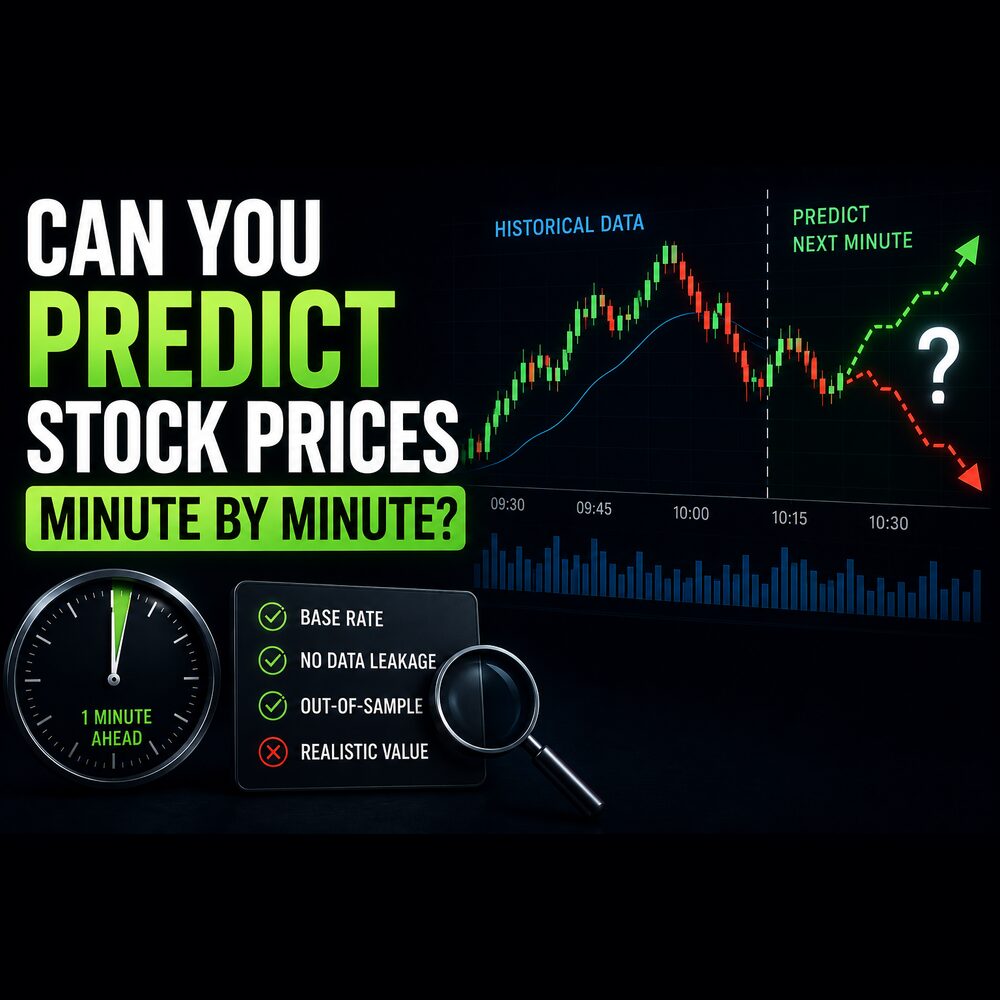
My best configuration was right 61.4% of the time on data it had never seen, against a market that went up in 46.8% of minutes. Roughly fifteen points of edge, on a model that only opens its mouth for 70 minutes out of 3,100. Whether that is a real edge or a well-dressed coin flip took four checks to work out, and the answer is not the one the headline number suggests.

The reason this is worth writing down is that a model can pass every test a tutorial teaches — held-out data, no lookahead in the features, a confusion matrix — and still be measuring nothing. The leak in mine was not in the features. It was in my process, and it does not show up as a train/validation gap, which is the only kind of overfitting most write-ups discuss.

The setup, briefly, so the numbers mean something: 9.4 million exchange records for 31 large companies, aggregated to one-minute bars, predicting whether the price is higher one minute later.

Check 0: the base rate

Before anything else, compute what a model has to beat. In my test period prices rose in 46.8% of minutes, so a program that ignores every input and always answers "up" is right 46.8% of the time. DummyClassifier builds that in one line and it belongs in the first row of every results table.

Class balance moves by asset and by period, so it has to be recomputed on the exact slice being reported. A model quoted at 58% accurate on a series that rises 57% of the time has done nothing at all, and that framing is missing from most published results — a 2019 study running standard models across the US market found accuracy distributed around 52% and statistically indistinguishable from chance, which is roughly what you would expect if the baseline were being quietly omitted.

Aggregation as a modelling decision

The raw data is trades — shares actually changing hands, 2.9 million of them — and quotes, the prices being advertised whether or not anyone accepted, another 6.4 million. Grouping by company and minute collapses that to about 11,600 rows with an open, high, low, close, volume and average spread each.

Going from 9.4 million records to 11,600 asserts that something predictable happens on a one-minute timescale and that everything faster is noise. Most of what you see tick by tick is the mechanics of order matching rather than information about direction, so I think the assertion is defensible here, but it is made before any modelling starts and no later result can rescue it if it is wrong.

Standard leakage: grouping and time-based splits

Labelling means pulling the closing price backwards by one row so each minute carries what happened next.

for horizon in horizons:                       # 1, 3 and 5 minutes ahead
    merged[f'future_price_{horizon}'] = (
        merged.groupby('company')['c'].shift(-horizon))

Without the groupby, the shift takes the first minute of one company's day and attaches it to the last minute of another's, inventing an answer from two unrelated series. The same trap exists in any panel data: users, sensors, regions.

The split has to be by time rather than at random, because neighbouring minutes share features computed from rolling windows, so a randomly chosen test row usually has its own neighbours sitting in training. I held back the last 100 minutes per company, which is 3,100 test rows across 31 companies. Features are averages and volatility of price and volume over the previous 3, 5, 10 and 20 minutes, computed per company and always backwards.

Both of those are necessary and neither is sufficient. Mine were correct and the result was still meaningless.

Check 1: tuning against the test set

The model outputs a confidence rather than a verdict, and you choose the level at which to act. Low, and you act often on weak signals; high, and you act rarely on strong ones. The natural move is to try several and keep the best.

for threshold in [0.5, 0.6, 0.65, 0.7]:
    preds = (probs > threshold).astype(int)
    precision = precision_score(y_test, preds, zero_division=0)
    print(f"Threshold: {threshold}, Precision: {precision:.4f}, Trades: {preds.sum()}")

At the middle setting the model acted 1,149 times and was right 47.95%, which is indistinguishable from always guessing up. That is the row that should have carried the most weight. At 0.6 it managed 50.8% over 327 attempts, and pushing higher made it worse than guessing. That shape — no monotonic improvement as confidence rises — says the confidence scores are not ranking anything, which I should have read as the answer rather than continuing.

The 61.4% came from a random forest at 0.63, and I picked 0.63 by looking at how it scored on the data I was using to judge it. Held-out data measures generalisation only for as long as you make no decisions based on it; once you tune against it, it measures how many things you tried. Nothing in my code leaked a future price. The leak was in the procedure, and the fix is a three-way split: one slice to learn from, a second to choose settings on, and a third opened exactly once. Bailey and López de Prado put numbers on this: try enough configurations against one holdout and a good-looking result is the expected outcome rather than evidence.

Check 2: sample size and decision count

Precision at threshold 0.63: 0.6143
Confusion Matrix:
[[1622   27]
 [1408   43]]
Predicted 1 count: 70
Actual 1 count: 1451

Seventy decisions out of 3,100 minutes. Forty-three right, twenty-seven wrong. With no skill you would expect about 33 right out of 70, so 43 is high, and with numbers this small that is roughly what coin flips give you when they fall your way. A binomial interval on 43/70 runs from about 49% to 73%. That contains the 46.8% base rate, so the data cannot rule out no skill at all — and it also reaches well past 61%, so it cannot rule out a real edge. Seventy decisions simply do not decide it.

The other direction of the matrix looks alarming and mostly is not. There were 1,451 minutes where the price rose and the model stayed silent for 1,408 of them, catching about 3% of what it was looking for. Low recall is not by itself a defect: a model that declines to answer 97.7% of the time and is right when it does speak is a perfectly reasonable design, and passing on an opportunity costs you nothing but the opportunity. The problem is not that it is selective. It is that 70 decisions cannot tell you whether the selection works.

Report the number of decisions alongside the rate, always, and treat any precision figure built on fewer than a few hundred as a hypothesis worth testing rather than a result.

Check 3: survival after costs

A percentage invites more tuning. Money does not. Simulating the strategy — fixed position size, every signal at the 0.6 setting, 327 trades — came out flat before costs and clearly negative once realistic brokerage and transaction taxes are applied to 327 round trips.

That is the 0.6 configuration, not the 61.4% one, and the distinction matters. The 0.63 setting fires a fifth as often, so it pays a fifth of the costs, and I have not run its profit and loss separately. What I can say is that a hit rate does not settle it either way, because direction says nothing about magnitude: 43 wins and 27 losses is profitable only if the average win is at least the size of the average loss, and on one-minute moves that is an assumption, not a result. Until that simulation exists, 61.4% is a hit rate and not a return.

That is the check worth running before any other, and it generalises past finance: convert the metric into the unit the decision is actually made in. Cost per false positive, hours of review per alert, money per round trip. An edge smaller than the friction is not an edge, and an accuracy figure will never tell you that on its own.

An evaluation checklist

Quote the base rate first, on the slice being reported. Split three ways so that every threshold and hyperparameter decision happens against data the final number never sees. Score on the decision unit from the beginning rather than optimising accuracy and checking profit afterwards — had I scored each threshold on net return, most of the range would have been visibly underwater on the first run.

Test across many periods rather than one. TimeSeriesSplit does this in about four lines, and reporting the spread across windows rather than a single number would have made the sample-size problem obvious immediately. For financial series specifically there is a subtlety I did not know about at the time: when labels are built from overlapping future windows, adjacent training and test rows share outcomes, and the standard fix is to purge the rows around the boundary and embargo a gap after it. López de Prado works through why, and it is the thing I would read first before attempting this again.

And match the test period to how often the model acts. If a setting fires 70 times across the whole window, the window is too short to judge it — either get more data or restrict yourself to settings that produce enough decisions to measure.

The pipeline underneath an inconclusive result is still worth keeping. Minute bars, a resumable backfill and a feature set are reusable whatever the model concludes, and making the collection safe to rerun turned out to be the part with lasting value.

References and further reading

Marcos López de Prado's Advances in Financial Machine Learning is the standard reference for testing models on financial data specifically, including the techniques for splitting time series so that overlapping windows cannot leak answers between the two halves. His chapters on how backtests mislead describe check 1 above almost exactly.

Bailey, Borwein, López de Prado and Zhu's The Probability of Backtest Overfitting puts numbers on the thing I did by hand: try enough configurations against one held-out period and a good-looking result is the expected outcome rather than evidence. It is the paper to read if you have ever tuned a threshold while watching the score.

The specific tools

• DummyClassifier — the baseline in one line. If your model does not clearly beat it, there is nothing to discuss.
• TimeSeriesSplit — testing across many periods instead of one, which is the smallest fix for the sample-size problem here.
• Precision-recall curve — plotted against the 46.8% baseline it shows in one picture what my table of confidence levels took several runs to reveal: most of the curve sits at or below the line you get for free.
• scikit-learn on cross-validation for time series — why a random split leaks when neighbouring rows share rolling-window features.

Related posts

• How to make an ETL pipeline safe to rerun — how the price data underneath a study like this gets collected, and re-collected safely.
• How to test a data pipeline — measuring how much a result moves on its own before comparing it to anything, in a testing setting.

My own projects

• Minute-level stock prediction — the pipeline and feature set behind this study, in more detail.
• Trader sentiment analysis — a smaller study on the same kind of data, with the baseline stated up front.
• Fraud detection — a model that does beat its baseline by a wide margin; the contrast with this one is the interesting part.